Suppose we integrate Eq. (8.19) over all velocities. The first term will become
 |
(8.21) |
The integral of the distribution function over velocities,
![]() is just the density of stars. And we're allowed to
interchange the integral over velocities, with the derivative wrt time,
since the range of velocities over which we integrate does not depend
on
is just the density of stars. And we're allowed to
interchange the integral over velocities, with the derivative wrt time,
since the range of velocities over which we integrate does not depend
on ![]() .
.
Integrating the second term, gives
| (8.22) |
where I've introduced the mean velocity ![]() as
as
 |
(8.23) |
Now the last term is zero, since
| (8.24) |
since there are no stars with infinite velocity.
And so the first moment of the CBE is a continuity equation for the density,
| (8.25) |
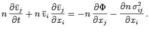
Now the second moment is what we're after. The trick is to first multiply the
CBE with ![]() , and then integrate over all velocities. The
calculation proceeds exactly as for the density, and the result is
after a bit of algebra:
, and then integrate over all velocities. The
calculation proceeds exactly as for the density, and the result is
after a bit of algebra:
| (8.26) |
where
| (8.27) |
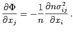
This was a lot of mathematics to come to a simple equation: suppose the
system is in a steady state,
 =0, and there are no
streaming motions, so that
=0, and there are no
streaming motions, so that
![]() . Then the previous equation
simplifies to
. Then the previous equation
simplifies to
| (8.28) |
This is a more general version for the equation of hydrostatic
equilibrium. To see this, note that the matrix
![]() is
symmetric:
is
symmetric:
![]() . For such symmetric tensors, we
can always rotate the coordinate system such that the tensor becomes
diagonal, i.e.
. For such symmetric tensors, we
can always rotate the coordinate system such that the tensor becomes
diagonal, i.e.
![]() for
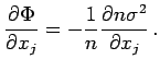
for ![]() . Now, suppose that the
velocities are isotropic, so that
. Now, suppose that the
velocities are isotropic, so that
![]() . Then we find that
. Then we find that
| (8.29) |
which is exactly the same as the equation for hydrostatic
equilibrium, if  is identified with the pressure
 ![]() .
Because of this analogy, the tensor
.
Because of this analogy, the tensor
![]() is called the
pressure tensor.
is called the
pressure tensor.
In conclusion: the behaviour of collisionless stellar systems is
similar to that of self-gravitating gas spheres. The role of
temperature is taken over by that of the stellar velocity dispersion.
It is the high velocity dispersion of the stars in an elliptical (and
also in the bulge of spirals), which balances the gravitational
pull. Since the required velocities are so high, such systems are
called `hot stellar systems'. Recall that in disk galaxies, it is
the ordered motion of the stars - i.e. the rotation of the disk -
which supports the system against gravity. Such systems are dynamically
cold, i.e. the stellar velocity dispersion is small compared to
the streaming motions. For disks, the `velocity dispersion' refers to the small velocities that stars have with respect to their
`local standard of rest' (10s of km s![]() ), versus the rotational
velocity of the disk, 200km s
), versus the rotational
velocity of the disk, 200km s![]() .
.
In a gas the pressure is isotropic and hence stars are spherical. In
contrast in stellar systems, the pressure tensor
![]() is
in general not isotropic, and so the pressure gradient can be
larger in one direction (
is
in general not isotropic, and so the pressure gradient can be
larger in one direction ( , say) than in another direction (
 ). So
even if the potential is spherical, the stellar distribution may be
more extended in than in , and the system will be elliptical in
shape.
). So
even if the potential is spherical, the stellar distribution may be
more extended in than in , and the system will be elliptical in
shape.