


 of the stars in an E-type galaxy with the total
luminosity
of the stars in an E-type galaxy with the total
luminosity  ,
,
Compare with the Tully-Fisher relation for spirals, Eq. (10.1):
the velocity dispersion takes the role of the circular
velocity  .
.
Comparison of Figure 10.3 with Figure 10.2 shows that
the scatter in the Faber-Jackson relation is quite a bit bigger
than the scatter in the Tully-Fisher relation: at a given value of
, there is a range of 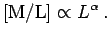 magnitudes in
  (i.e. a
factor 2.5 in ), versus a few tenths of a magnitude for a given
value of in the Tully-Fisher relation. So ellipticals follow a
similar relation as spirals, with more luminous and hence more massive,
ellipticals having a large velocity dispersion, but the relation is not
as tight as the corresponding
(i.e. a
factor 2.5 in ), versus a few tenths of a magnitude for a given
value of in the Tully-Fisher relation. So ellipticals follow a
similar relation as spirals, with more luminous and hence more massive,
ellipticals having a large velocity dispersion, but the relation is not
as tight as the corresponding  relation in spirals.
 |
From all the parameters we can measure for an elliptical, the total
luminosity , the velocity dispersion , the effective radius
 and the intensity
  (which both enter in the de Vaucouleurs
profile, Eq. (3.2)), only three are independent. So we can try
to obtain a tighter relation by introducing a second parameter in
Eq. (10.7), for example . This is how it goes: suppose that
the galaxy is in virial equilibrium, then its kinetic energy
(which both enter in the de Vaucouleurs
profile, Eq. (3.2)), only three are independent. So we can try
to obtain a tighter relation by introducing a second parameter in
Eq. (10.7), for example . This is how it goes: suppose that
the galaxy is in virial equilibrium, then its kinetic energy
 will be proportional to its potential energy
  ,
and so we expect
,
and so we expect
 |
(10.8) |
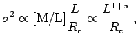
Introducing again the mass-to-light ratio, [M/L] this can be written as
![$\displaystyle \sigma^2 \propto \hbox{[M/L]}{L\over R_e} \propto {L^{1+\alpha}\over R_e}\,,$](img655.png) |
(10.9) |
where I've assumed [M/L] to depend on as
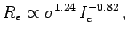
The intensity
 , hence
 |
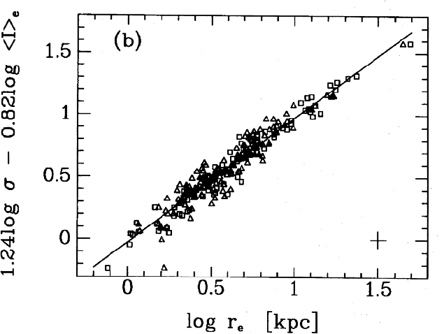
Figure 10.4 shows that
for the same sample of ellipticals which was plotted in
Figure 10.3. The galaxies follow this relation with very little
scatter. Comparing the last two equations shows that if we assume
 , then
 -
very nearly the same as what the figure suggests. Put differently, if
the mass-to-light ratio of ellipticals depends on luminosity as
-
very nearly the same as what the figure suggests. Put differently, if
the mass-to-light ratio of ellipticals depends on luminosity as
 , then we can understand why ellipticals follow
the relation plotted in Figure 10.4 so tightly.
, then we can understand why ellipticals follow
the relation plotted in Figure 10.4 so tightly.
The relation Eq. (10.12) is called the fundamental plane
of elliptical galaxies. In four dimensional , , and
space, galaxies do not occupy the whole space, but are restricted
to a 3-dimensional surface defined by relation (10.12), hence
the name fundamental plane.
 for a sample of elliptical
galaxies plotted versus the velocity dispersion
for a sample of elliptical
galaxies plotted versus the velocity dispersion  ). Brighter ellipticals galaxies (more negative
 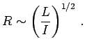 +constant) have a larger velocity dispersion.
![$\displaystyle \hbox{[M/L]}\propto L^\alpha\,.$](img656.png)

 for the
same sample of Es plotted in Figure
for the
same sample of Es plotted in Figure 