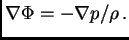
(This should look familiar from hydrostatic equilibrium in stars!) By
modelling the spectrum as function of position, we can determine  and
and
 separately, and hence the rhs of Eq.(6.7). From that,
one can reconstruct the gravitational potential, and hence infer the
mass distribution.
separately, and hence the rhs of Eq.(6.7). From that,
one can reconstruct the gravitational potential, and hence infer the
mass distribution.
The temperature is observed to remain approximately constant, in
which case we can obtain an approximate expression for the density
profile. The pressure is
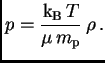 |
(6.8) |
If we take constant then the rhs of Eq. (6.7) becomes
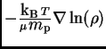 . The lhs of this equation
is just the gravitational force,
. The lhs of this equation
is just the gravitational force,
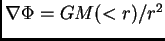 , with
  the mass interior to
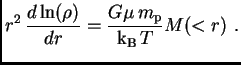
  . Combining
these two, we obtain after some rearranging
. Combining
these two, we obtain after some rearranging
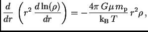
Taking the derivative of both sides with respect to  , gives
since
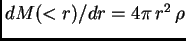 . Try a solution of the form
 , where
  and
and  are constants. Substituting this, the
lhs of Eq. (6.10) is , and the rhs is
are constants. Substituting this, the
lhs of Eq. (6.10) is , and the rhs is
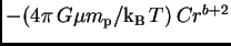 . If this is to be a solution,
then
. If this is to be a solution,
then  , and
, and
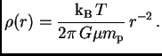 |
(6.11) |
This would be the density profile if the gas were to furnish the
gravitational potential required to keep it in hydrostatic
equilibrium. However, in addition to the gas, there is also the
gravitational potential due to stars. And so we should have used
 . By estimating the mass
in stars, we can correct our density distribution to what it should be,
in the presence of stars. Since this extra gravity increases the rhs of
Eq. (6.9), the density
. By estimating the mass
in stars, we can correct our density distribution to what it should be,
in the presence of stars. Since this extra gravity increases the rhs of
Eq. (6.9), the density
 will need to increase
as well.
will need to increase
as well.
Given the corrected density profile, we can compute the expected X-ray
emissivity, since that depends on the density
 . The emissivity is much higher than expected, and hence we
infer the presence of dark matter in ellipticals.
. The emissivity is much higher than expected, and hence we
infer the presence of dark matter in ellipticals.